AIS Data and Graph Construction

Objectives

• Understand the Automatic Identification System (AIS) and its role in maritime monitoring

• Know why velocity, distance to shore, and curvature are discriminative features

• Understand the graph construction code that converts numpy arrays to DGL graphs

• Know the dataset statistics and bootstrap split methodology

AIS Data Availability

AIS data is one of the most accessible sources of maritime intelligence. The International Maritime Organization (IMO) requires all vessels over 300 gross tons on international voyages to carry AIS transponders. In Norwegian waters, the Norwegian Coastal Administration provides historical AIS data through kystverket.no, and global AIS feeds are available from providers like MarineTraffic and Spire. This demonstrator uses pre-processed AIS data from Norwegian coastal waters, where fishing activity is a significant component of vessel traffic.

Automatic Identification System (AIS)

AIS is a maritime tracking system originally designed for collision avoidance. Vessels broadcast their position and status at regular intervals (every 2-30 seconds depending on speed). Each AIS message contains:

Field	Description	Update Rate
MMSI	Unique vessel identifier	Static
Position (lat, lon)	GPS coordinates	2-30 seconds
Speed over ground (SOG)	Vessel speed in knots	2-30 seconds
Course over ground (COG)	Direction of travel	2-30 seconds
Heading	Direction the bow points	2-30 seconds
Vessel type	Ship category code	Static
Navigation status	Underway, anchored, fishing, etc.	Variable

For classification purposes, raw AIS messages are aggregated into fixed-length time-series segments representing vessel behavior over a defined time window.

Feature Engineering

From raw AIS data, three features are extracted for each of the 12 time steps. These features were chosen because they capture distinct aspects of fishing behavior:

Feature	Description	Why It Is Discriminative
Velocity	Speed of the vessel (derived from SOG)	Fishing vessels typically operate at lower and more variable speeds than transit vessels. Trawlers maintain 2-5 knots while dragging nets, compared to 10-15 knots for transit. Speed variability is also higher during fishing as vessels adjust to catch conditions.
Distance to shore	Proximity to the coastline	Fishing often occurs in specific zones – continental shelves, banks, and areas with known fish aggregations. Coastal fishing vessels operate within 12-50 nautical miles, while transit vessels often take more direct offshore routes.
Curvature	Rate of course change (derived from COG differences)	Fishing involves more frequent and sharper turns than transit. Vessels circling fish schools, setting longlines, or trawling in patterns produce high curvature values. Transit vessels maintain nearly straight courses with curvature close to zero.

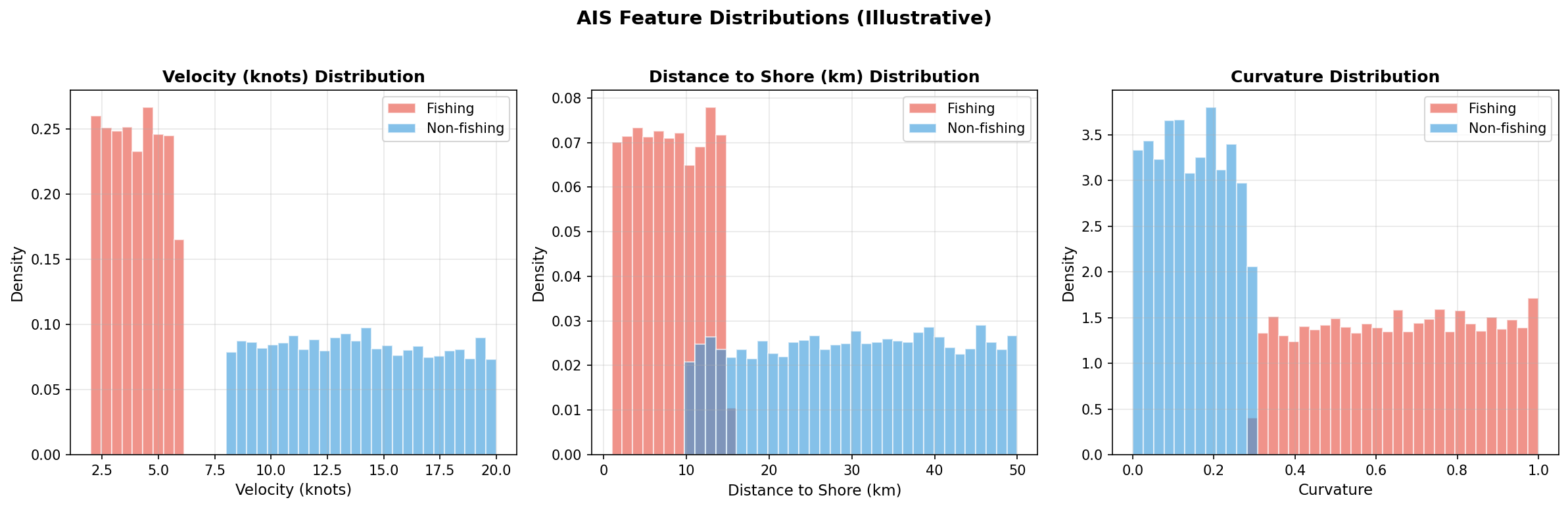
Distribution of the three features for fishing (orange) and non-fishing (blue) vessel trajectories. Fishing vessels show lower, more variable speeds; closer proximity to shore; and higher trajectory curvature.

Graph Construction Code

The AISTimeseriesDataset class in src/graph_classification/ais_timeseries_dataset.py converts numpy arrays to DGL graphs. Here is the core graph construction logic:

import dgl
import torch
import numpy as np

def build_graph_from_features(features, num_timesteps=12):
    """Convert a single AIS trajectory to a DGL graph.

    Args:
        features: numpy array of shape (3, 12) -- 3 features x 12 time steps
        num_timesteps: number of time steps (nodes in the graph)

    Returns:
        DGL graph with node features and self-loops
    """
    # Create sequential edges: 0->1, 1->2, ..., 10->11
    edge_list = [(i, i + 1) for i in range(num_timesteps - 1)]

    # Transpose features to (12, 3) -- one row per node
    node_features = torch.tensor(features.T, dtype=torch.float32)

    # Create the DGL graph
    graph = dgl.graph(edge_list)

    # Assign node features
    graph.ndata['attr'] = node_features

    # Add self-loops to avoid 0-in-degree errors during message passing
    graph = dgl.add_self_loop(graph)

    return graph

Each constructed graph has the following structure:

Property	Value
Nodes	12 (one per time step)
Sequential edges	11 (chain: 0-1, 1-2, …, 10-11)
Self-loop edges	12 (one per node)
Total edges	23
Node feature dimension	3 (velocity, distance to shore, curvature)

The full dataset is loaded and converted in batch by the AISTimeseriesDataset class, which extends DGLDataset and handles caching, saving, and loading of the graph objects.

Dataset Statistics

The dataset contains approximately 23,500 AIS trajectory samples collected from Norwegian coastal waters:

Split	Samples	Percentage	Purpose
Training	14,100	60%	Model training
Validation	4,700	20%	Hyperparameter tuning, early stopping
Test	4,700	20%	Final evaluation
Total	~23,500	100%

Class Distribution

The dataset is approximately balanced between the two classes:

Class	Label	Description
Non-fishing	0	Transit, anchored, maneuvering, or other non-fishing activities
Fishing	1	Active fishing operations (trawling, longlining, purse seining, etc.)

Data Format

The raw data is stored as three numpy files:

import numpy as np

# Features: (N, 3, 12) -- N samples, 3 features, 12 time steps
X = np.load('data/X_ts12.npy')
print(f'Features shape: {X.shape}')  # (23500, 3, 12)

# Labels: (N,) -- binary classification
y = np.load('data/y_ts12.npy')
print(f'Labels shape: {y.shape}')    # (23500,)
print(f'Class distribution: {np.bincount(y.astype(int))}')

# Bootstrap indices: (50, N) -- 50 different splits
bidx = np.load('data/bidx_ts12.npy')
print(f'Bootstrap shape: {bidx.shape}')  # (50, 23500)

Bootstrap Split Methodology

The dataset includes 50 pre-computed train/val/test splits (bootstrap indices) to enable robust evaluation. Each split assigns every sample one of three roles:

Index Value	Role	Description
1	Training	Used for model weight updates
2	Validation	Used for early stopping and hyperparameter selection
3	Test	Used for final accuracy reporting

Using the --bootstrap_index N flag (0-49) selects a specific split. When no bootstrap index is specified (default), a combined split is used. Running experiments across multiple bootstrap indices provides confidence intervals for the reported accuracy.

Keypoints

• AIS is a mandatory maritime tracking system that provides position, speed, and course data

• Three features are extracted: velocity, distance to shore, and curvature – each captures a different aspect of fishing behavior

• Each trajectory is converted to a chain graph with 12 nodes, 11 sequential edges, and 12 self-loops

• The dataset contains ~23,500 samples with approximately balanced classes

• 50 bootstrap splits enable robust evaluation with confidence intervals

• The AISTimeseriesDataset class handles conversion from numpy arrays to DGL graphs with caching