Running the Demonstrator

Objectives

Run the demonstrator via Jupyter notebook or command line
Understand the training script arguments and their effects
Interpret the accuracy results across models and learning rates
Tune hyperparameters: learning rate, epochs, batch size, and patience
Use bootstrap indices for robust evaluation

Option A: Jupyter Notebook

The interactive notebook provides visualizations, inline plots, and step-by-step execution.

Starting Jupyter

cd ~/graph-based-classification-of-ais-time-series-data
source venv/bin/activate
jupyter lab --no-browser --ip=127.0.0.1 --port=8888

If running on a remote VM, set up an SSH tunnel to access the notebook locally:

# On your local machine
ssh -L 8888:localhost:8888 -i ~/.ssh/naic-vm.pem ubuntu@<YOUR_VM_IP>

Then open http://localhost:8888 in your browser.

Running the Notebook

Open notebooks/DGL_Demonstrator.ipynb
Select the ais_dgl kernel from the kernel dropdown
Run all cells (Kernel > Restart Kernel and Run All Cells)

The notebook trains GCN, GraphSAGE, and GAT models, evaluates them on the test set, and displays performance comparison plots including training curves and accuracy bar charts.

Kernel Not Found?

If the ais_dgl kernel is not available, register it manually:

python -m ipykernel install --user --name=ais_dgl --display-name "AIS DGL (Python 3)"

Then restart Jupyter Lab and select the new kernel.

Option B: Command Line

The training script provides full control over models, hyperparameters, and evaluation.

Training All Models

cd ~/graph-based-classification-of-ais-time-series-data
source venv/bin/activate
export PYTHONPATH=$PYTHONPATH:$(pwd)/src

# Train all three models with default settings
python src/graph_classification/train_graph_classification_ais.py \
    --data_folder data/ \
    --model_path results/ \
    --models "GCN, GSG, GAT" \
    --epochs 100 \
    --patience 20

Quick Test (Recommended First)

Run a few epochs to verify everything works before committing to a full training run:

python src/graph_classification/train_graph_classification_ais.py \
    --data_folder data/ \
    --model_path results/ \
    --models "GCN" \
    --epochs 10 \
    --patience 5

Command Line Options

Option	Default	Description
`--data_folder`	`../data/`	Path to directory containing `.npy` data files
`--model_path`	`../results`	Directory for saving trained models and results
`--models`	`"GCN, GSG, GAT"`	Comma-separated list of models to train
`--gpu`	`0`	GPU device index (`-1` for CPU)
`--lrs`	`"5e-2, 3e-2, 1e-2"`	Comma-separated learning rates to iterate over
`--epochs`	`1000`	Maximum number of training epochs
`--hidden`	`32`	Size of hidden layers
`--batch_size`	`600`	Batch size for data loading
`--patience`	`200`	Early stopping patience (epochs without improvement)
`--bootstrap_index`	`None`	Bootstrap split index (0-49), or None for combined split
`--pin_memory`	`True`	Pin memory for faster GPU data transfer
`--num_workers`	`0`	Number of data loading workers

Evaluation

After training, evaluate saved models on the test set:

python src/graph_classification/eval_graph_classification_ais.py \
    --data_folder data/ \
    --model_path results/

Understanding the Results

Accuracy Table

The demonstrator produces a comparison table across models and learning rates:

Model	Learning Rate	Test Accuracy
GCN	0.010	94.4%
GraphSAGE (GSG)	0.010	94.4%
GAT	0.010	93.1%
GCN	0.025	94.2%
GraphSAGE (GSG)	0.025	94.4%
GAT	0.025	86.3%

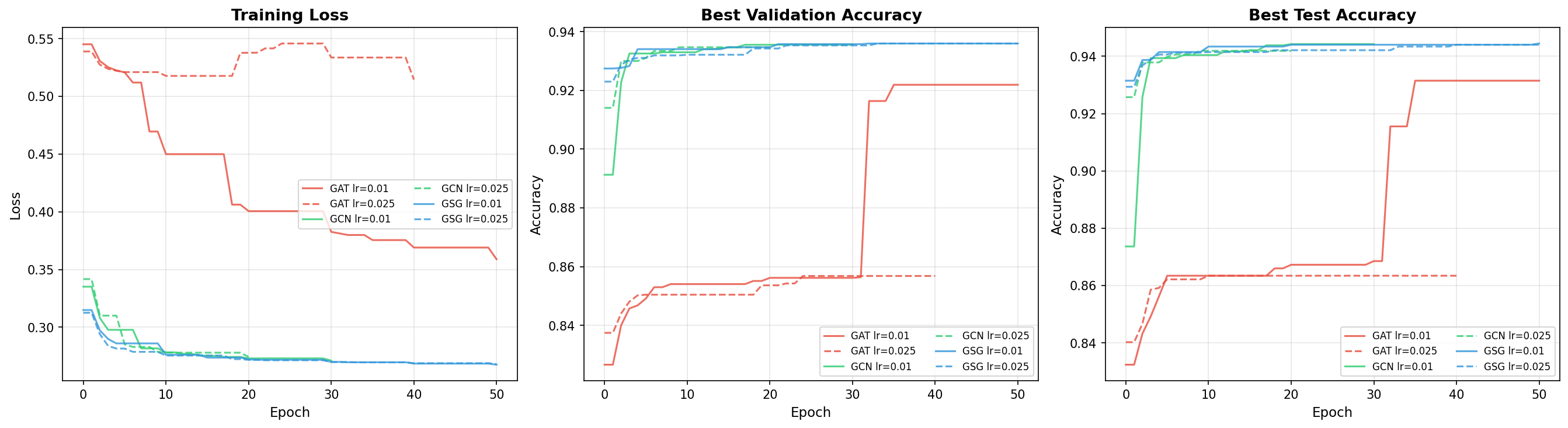
Training loss and validation accuracy curves for GCN, GraphSAGE, and GAT — Training curves for the three GNN architectures. GraphSAGE converges smoothly and maintains high accuracy across different learning rates. GAT shows more variability, particularly at higher learning rates.

Interpreting the Numbers

GCN (94.4%): Strong baseline performance. The degree-normalized aggregation is well-suited to the regular chain graph structure where all nodes have similar degree.

GraphSAGE (94.4%): Matches GCN at the best learning rate and is more robust to learning rate changes. At lr=0.025, GraphSAGE still achieves 94.4% while GCN drops slightly to 94.2%. This consistency makes GraphSAGE the recommended model for production use.

GAT (93.1% at lr=0.01, 86.3% at lr=0.025): Slightly lower accuracy and significantly more sensitive to learning rate. At lr=0.025, GAT drops to 86.3% – an 8-point decline. The attention mechanism adds parameters and complexity that may not be necessary for the regular chain graph structure. The dropout (0.5) in GAT layers also introduces additional training variance.

What 94.4% Accuracy Means

On the test set of ~4,700 samples:

~4,436 samples are correctly classified
~264 samples are misclassified
This includes both false positives (non-fishing classified as fishing) and false negatives (fishing classified as non-fishing)

For maritime monitoring applications, the false negative rate (missed fishing activity) is typically more critical than the false positive rate. Further analysis of the confusion matrix can guide threshold tuning.

Parameter Tuning

Learning Rate

The learning rate has the largest impact on training dynamics:

Learning Rate	Effect
0.001	Very slow convergence; may need 500+ epochs to reach optimal accuracy
0.010	Good balance of speed and stability; recommended starting point
0.025	Faster convergence but riskier; works well for GCN/GraphSAGE, can destabilize GAT
0.050	Aggressive; may cause oscillation or divergence, especially for GAT

Epochs and Patience

Epochs: Maximum training duration. Default is 1000, but early stopping usually triggers much sooner.
Patience: Number of epochs without validation improvement before stopping. Lower patience (20-50) gives faster training but may stop too early. Higher patience (100-200) allows more exploration but uses more compute.

Recommended combinations:

Scenario	Epochs	Patience
Quick test	10-20	5
Standard training	100	20
Thorough training	500	50
Full exploration	1000	200

Batch Size

Smaller batches (100-300): More parameter updates per epoch, noisier gradients, can escape local minima
Default (600): Good balance for the dataset size (~14,100 training samples)
Larger batches (2000-4000): Faster epoch time on GPU, smoother gradients, may converge to sharper minima

If you encounter CUDA out-of-memory errors, reduce the batch size:

python src/graph_classification/train_graph_classification_ais.py \
    --data_folder data/ \
    --batch_size 200 \
    --epochs 100

Bootstrap Indices

The dataset includes 50 pre-computed train/val/test splits to enable robust evaluation. Use the --bootstrap_index flag to select a specific split:

# Train on bootstrap split 0
python src/graph_classification/train_graph_classification_ais.py \
    --data_folder data/ \
    --model_path results/ \
    --models "GSG" \
    --bootstrap_index 0 \
    --epochs 100

# Train on bootstrap split 1
python src/graph_classification/train_graph_classification_ais.py \
    --data_folder data/ \
    --model_path results/ \
    --models "GSG" \
    --bootstrap_index 1 \
    --epochs 100

When --bootstrap_index is not specified (default), a combined split is used where any sample assigned to training in any of the 50 splits is used for training.

Running across multiple splits (e.g., 0-9) and averaging the test accuracy provides a more robust performance estimate with confidence intervals. This is particularly useful when comparing architectures or hyperparameter settings.

Background Training

For long-running experiments, use tmux to keep the training alive after disconnecting:

# Start a new tmux session
tmux new -s gnn-training

# Inside tmux, run training
cd ~/graph-based-classification-of-ais-time-series-data
source venv/bin/activate
export PYTHONPATH=$PYTHONPATH:$(pwd)/src
python src/graph_classification/train_graph_classification_ais.py \
    --data_folder data/ \
    --model_path results/ \
    --models "GCN, GSG, GAT" \
    --epochs 500 \
    --patience 50 2>&1 | tee training.log

# Detach from tmux: Ctrl+B, then D
# Reattach later: tmux attach -t gnn-training

Results are saved to results/ais_classification_model_results.json with per-model accuracy scores.

Keypoints

Use the Jupyter notebook for interactive exploration and visualization
Use the CLI for reproducible, scriptable training runs
GraphSAGE achieves the best and most consistent results (94.4%) across learning rates
GAT is sensitive to learning rate – use lr=0.01 to avoid instability
Start with a quick test (10 epochs) before running full training
Bootstrap indices (0-49) enable robust evaluation across different data splits
Use tmux for long-running training on remote VMs
Lower batch size if you encounter CUDA out-of-memory errors
Patience controls early stopping – lower values (20) for speed, higher values (200) for thorough exploration