Understanding the SHGA Algorithm

Objectives

• Understand the two-phase hybrid approach

• Learn how deterministic crowding maintains diversity

• Understand how CMA-ES refines solutions

• Know how to configure algorithm parameters

Why This Matters

The Scenario: A process engineer running a chemical reactor knows there are multiple operating points that maximize yield — different temperature-pressure-flow combinations that all produce good results. A standard optimizer converges to whichever optimum it stumbles on first, but she needs all of them so operators can switch between regimes depending on feedstock availability.

The Research Question: How does deterministic crowding prevent a genetic algorithm from collapsing onto a single optimum, and how does the two-phase seed-solve-collect cycle combine global exploration with high-precision local refinement?

What This Episode Gives You: The algorithm internals — GA with niching, CMA-ES local search, and how to configure budget, population size, and convergence tolerances.

Algorithm Overview

The Scalable Hybrid Genetic Algorithm (SHGA) uses a seed-solve-collect paradigm:

        flowchart LR
    A[Initialize Population] --> B[Deterministic Crowding GA]
    B --> C[Extract Seeds]
    C --> D[CMA-ES Local Search]
    D --> E[Collect Solutions]
    E --> F{Budget Exhausted?}
    F -->|No| B
    F -->|Yes| G[Return All Solutions]
    

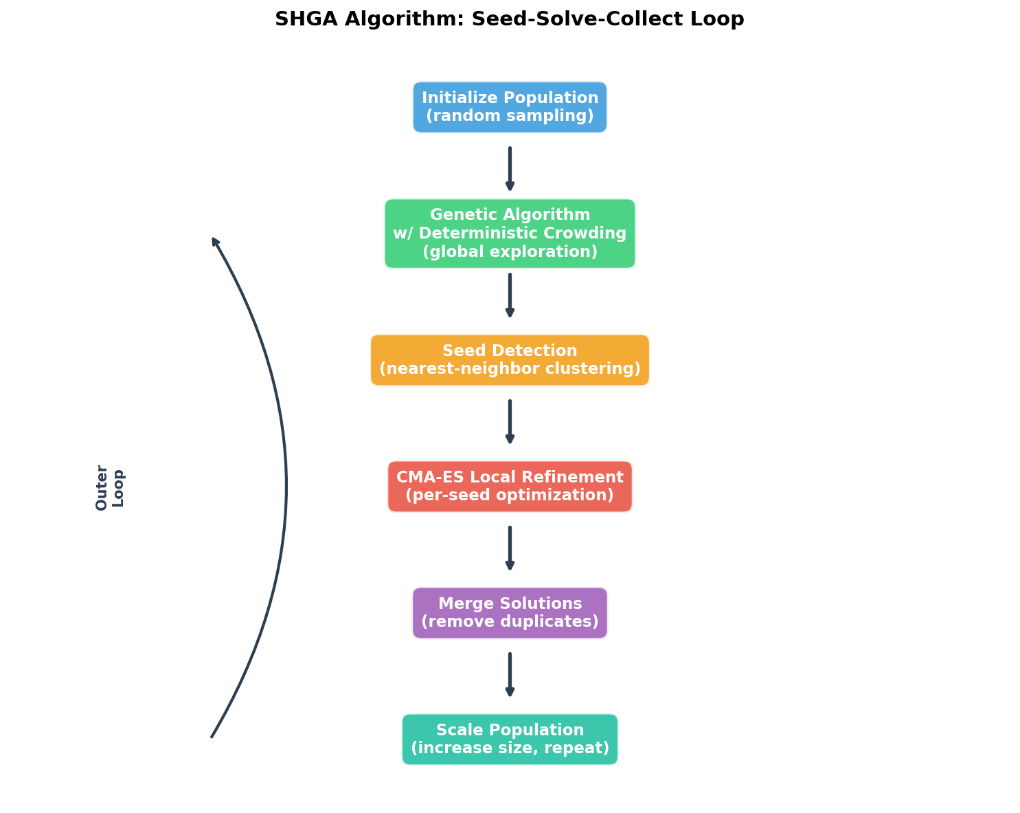
The SHGA algorithm iterates through initialization, genetic algorithm exploration, seed detection, CMA-ES local refinement, solution merging, and population scaling.

Phase 1: Global Search (Deterministic Crowding GA)

The first phase explores the entire search space using a genetic algorithm with deterministic crowding:

1. Population Initialization: Random points sampled uniformly in the domain

2. Selection: Tournament selection for parent pairs

3. Crossover: BLX-alpha blend crossover

4. Mutation: Gaussian mutation with adaptive step size

5. Replacement: Child replaces most similar parent (deterministic crowding)

Why Deterministic Crowding? Standard GAs converge to a single optimum. Deterministic crowding maintains niches - subpopulations around different optima - by ensuring children only compete with similar parents.

Phase 2: Local Refinement (CMA-ES)

After the GA identifies promising regions, CMA-ES (Covariance Matrix Adaptation Evolution Strategy) refines each seed to high precision:

• Adaptive step size: Automatically adjusts search radius

• Covariance learning: Learns the local landscape shape

• Invariance properties: Works well regardless of coordinate system

CMA-ES is widely considered the state-of-the-art for local optimization in continuous spaces.

The Seed-Solve-Collect Cycle

Each iteration:

1. Seed: Extract promising candidates from GA population

2. Solve: Run CMA-ES from each seed

3. Collect: Add converged solutions to the solution set

This continues until the function evaluation budget is exhausted.

Key Algorithm Components

MultiModalMinimizer Class

The main entry point is mmo.minimize.MultiModalMinimizer:

from mmo.minimize import MultiModalMinimizer
from mmo.domain import Domain

# Define search domain
domain = Domain(boundary=[[-5, -5], [5, 5]])  # 2D box

# Create optimizer
optimizer = MultiModalMinimizer(
    f=my_function,        # Function to minimize
    domain=domain,        # Search space
    budget=50000,         # Max function evaluations
    max_iter=50,          # Max outer iterations
    verbose=1             # Output level (0-3)
)

# Run optimization
for result in optimizer:
    print(f"Iteration {result.number}: {result.n_sol} solutions found")

# Get all solutions
solutions = optimizer.xy  # Shape: (n_solutions, dim+1)
x_values = solutions[:, :-1]  # Solution coordinates
f_values = solutions[:, -1]   # Function values

Domain Class

Defines an axis-parallel hypercuboid search space:

from mmo.domain import Domain

# 2D domain: x in [-5, 5], y in [-5, 5]
domain_2d = Domain(boundary=[[-5, -5], [5, 5]])

# 10D domain: each dimension in [0, 1]
domain_10d = Domain(boundary=[[0]*10, [1]*10])

Configuration

Algorithm parameters are controlled via mmo.config.Config:

Parameter	Default	Description
n_pop	100	GA population size
n_gen	50	GA generations per iteration
p_c	0.9	Crossover probability
p_m	0.1	Mutation probability
sigma	0.5	CMA-ES initial step size
tol	1e-8	CMA-ES convergence tolerance

Algorithm Parameters

Choosing Budget

The budget (max function evaluations) depends on:

• Dimension: Higher dimensions need more budget

• Number of optima: More optima need more exploration

• Function cost: Expensive functions may need smaller budgets

CEC2013 recommended budgets:

Functions	Dimension	Optima	Budget
F1-F5	1-2D	1-5	50,000
F6-F7	2D	18-36	200,000
F8-F20	2-20D	6-216	400,000

Verbosity Levels

Level	Output
0	Silent
1	Summary per iteration
2	+ GA details
3	+ CMA-ES details

Keypoints

• SHGA combines genetic algorithm (global) with CMA-ES (local)

• Deterministic crowding maintains population diversity around multiple optima

• The seed-solve-collect cycle iteratively refines solutions

• Budget scales with dimension and number of expected optima