CEC2013 Benchmark Functions

Objectives

• Understand the CEC2013 multi-modal benchmark suite

• Know the characteristics of each function

• Learn how to use benchmarks for testing

Why This Matters

The Scenario: A benchmarking team at a research lab has developed a new multi-modal optimizer and wants to publish results. Reviewers will ask: how does it compare to the state of the art, and on which standard test problems? Without a recognized benchmark suite, every paper invents its own test functions, making comparison impossible.

The Research Question: What is the CEC2013 niching benchmark suite, what makes each of its 20 functions challenging in different ways, and what does a “good” Peak Ratio score actually mean?

What This Episode Gives You: The complete benchmark catalog — function properties, recommended budgets, evaluation code, and how to interpret your results against the standard.

Overview

The CEC2013 benchmark suite is the standard for evaluating multi-modal optimization algorithms. It includes 20 functions with varying:

• Dimensions: 1D to 20D

• Number of optima: 2 to 216

• Basin sizes: Equal to highly unequal

• Global/local structure: Some have only global optima, others have many local optima

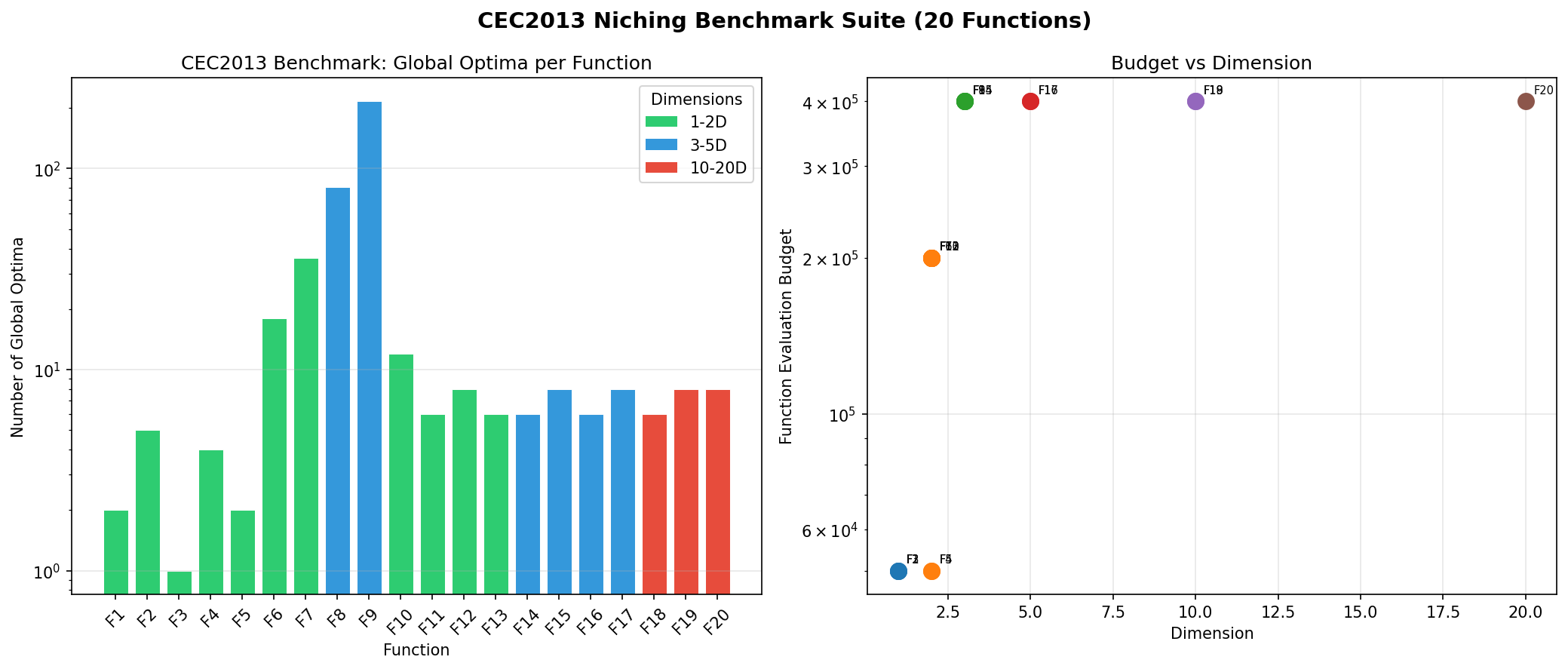
The CEC2013 suite spans 20 functions from 1D to 20D, with 1 to 216 global optima. Colors indicate dimensionality: green (1-2D), blue (3-5D), red (10-20D).

Function Catalog

Low-Dimensional (1-2D)

ID	Name	Dim	Global Optima	Budget
F1	Five-Uneven-Peak Trap	1	2	50,000
F2	Equal Maxima	1	5	50,000
F3	Uneven Decreasing Maxima	1	1	50,000
F4	Himmelblau	2	4	50,000
F5	Six-Hump Camel Back	2	2	50,000
F6	Shubert	2	18	200,000
F7	Vincent	2	36	200,000

Composition Functions (2-20D)

ID	Name	Dim	Global Optima	Budget
F8	Modified Rastrigin - All Global	2	12	400,000
F9	Composition Function 1	2	6	400,000
F10	Composition Function 2	2	8	400,000
F11	Composition Function 3	2	6	200,000
F12	Composition Function 4	3	8	400,000
F13-F20	Higher Dimensional	3-20	6-216	400,000

Using Benchmarks

Loading a Function

from cec2013.cec2013 import CEC2013, how_many_goptima
import numpy as np

# Load Himmelblau function (F4)
f = CEC2013(4)

# Get function information using direct methods
dim = f.get_dimension()
n_optima = f.get_no_goptima()
f_best = f.get_fitness_goptima()
budget = f.get_maxfes()

print(f"Name: Himmelblau (F4)")
print(f"Dimension: {dim}")
print(f"Number of global optima: {n_optima}")
print(f"Global optimum value: {f_best}")
print(f"Recommended budget: {budget}")

# Get bounds (must iterate over dimensions)
lb = [f.get_lbound(k) for k in range(dim)]
ub = [f.get_ubound(k) for k in range(dim)]
print(f"Lower bounds: {lb}")
print(f"Upper bounds: {ub}")

# Evaluate function
x = np.array([3.0, 2.0])  # Near one of the optima
value = f.evaluate(x)
print(f"f({x}) = {value}")

Checking Found Optima

# Use how_many_goptima to check found solutions
solutions = np.array([[3.0, 2.0], [-2.8, 3.1]])  # Example solutions
accuracy = 0.0001
count, seeds = how_many_goptima(solutions, f, accuracy)
print(f"Found {count}/{n_optima} global optima")

Function Details

F1: Five-Uneven-Peak Trap (1D)

• Domain: [0, 30]

• 5 peaks with different heights and widths

• 2 global optima at x = 0 and x = 30

F4: Himmelblau (2D)

• Domain: [-6, 6]^2

• Classic test function with 4 global optima

• Located at approximately:

  • (3.0, 2.0)

  • (-2.805, 3.131)

  • (-3.779, -3.283)

  • (3.584, -1.848)

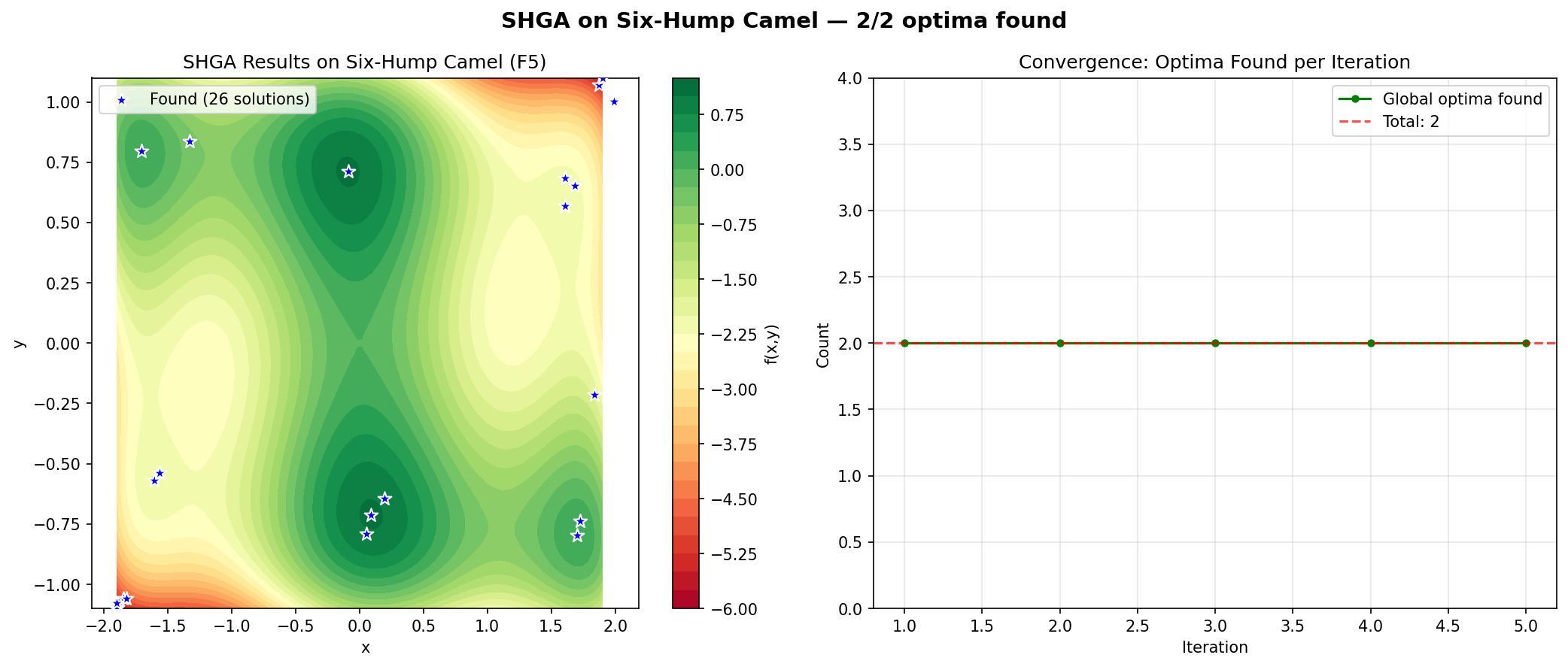
SHGA on the Six-Hump Camel (F5) — both global optima found with rapid convergence.

F6: Shubert (2D)

• Domain: [-10, 10]^2

• 760 local optima, 18 global optima

• All global optima have the same function value

• Tests ability to find many optima

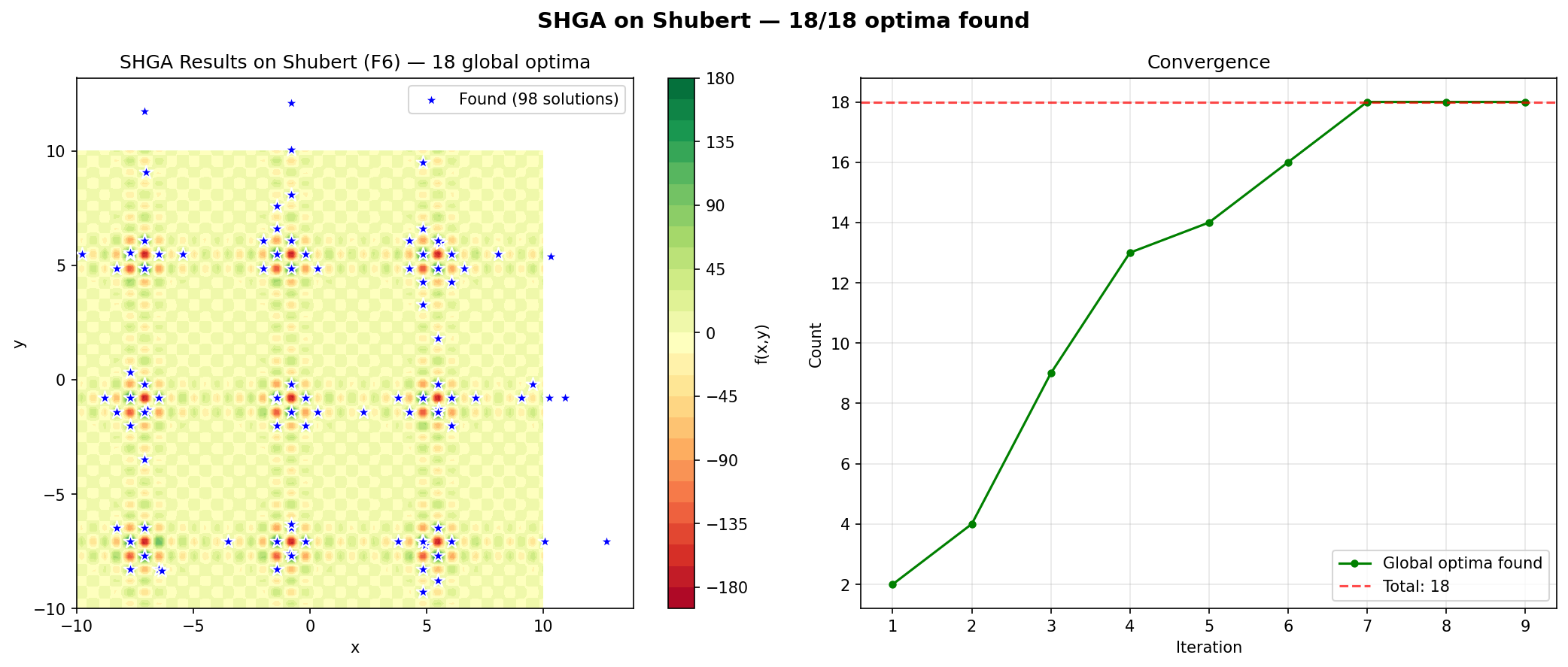
SHGA on the Shubert function (F6) — the algorithm must find 18 global optima scattered across a complex landscape with 760 local optima.

F7: Vincent (2D)

• Domain: [0.25, 10]^2

• 36 global optima in a regular pattern

• Each optimum in a separate basin

• Tests systematic coverage of the domain

Performance Metrics

Peak Ratio (PR)

The standard metric for multi-modal optimization:

PR = (Number of found global optima) / (Total known global optima)

A solution is “found” if it’s within accuracy threshold of a true optimum:

Accuracy Level	Distance Threshold
1e-1	0.1
1e-2	0.01
1e-3	0.001
1e-4	0.0001
1e-5	0.00001

Computing PR with CEC2013

The CEC2013 module provides how_many_goptima() to compute the peak ratio:

from cec2013.cec2013 import CEC2013, how_many_goptima

# After running optimizer...
f = CEC2013(4)  # Himmelblau
n_optima = f.get_no_goptima()

# Get found solutions (without function values)
found_solutions = optimizer.xy[:, :-1]

# Compute how many global optima were found
accuracy = 0.0001  # Distance threshold
count, seeds = how_many_goptima(found_solutions, f, accuracy)

# Peak ratio
pr = count / n_optima
print(f"Found {count}/{n_optima} global optima")
print(f"Peak Ratio: {pr:.2%}")

Choosing Functions for Testing

Purpose	Recommended Functions
Quick testing	F4 (Himmelblau), F5 (Six-Hump Camel)
Many optima	F6 (Shubert), F7 (Vincent)
Scalability	F11-F20 (higher dimensions)
Algorithm comparison	F1-F7 (standard benchmark)

Keypoints

• CEC2013 provides 20 standardized benchmark functions

• Functions range from 1D to 20D with 1 to 216 optima

• Peak Ratio (PR) is the standard performance metric

• Use F4 (Himmelblau) for quick testing

• Higher functions (F8+) test scalability to more dimensions