Analyzing Results

Objectives

• Load and interpret optimization results

• Compute performance metrics

• Visualize solutions and convergence

Why This Matters

The Scenario: An R&D manager reviews the optimization results and sees “32 solutions found.” But the benchmark has 36 known optima. She asks: did we find everything, or are we missing solutions in hard-to-reach regions? She needs a clear metric and visualization to answer this — not just a count, but a measure of completeness across accuracy levels.

The Research Question: How do you quantify the quality of a multi-modal optimizer’s output — distinguishing “found most optima approximately” from “found all optima precisely” — and how do you visualize where solutions are and where gaps remain?

What This Episode Gives You: The analysis toolkit — Peak Ratio computation, convergence plots, 2D solution visualization, and a systematic approach to diagnosing when and why the optimizer misses optima.

Loading Results

If you saved results as shown in Episode 05:

import pandas as pd
import numpy as np
import json

# Load experiment results
exp_dir = "results/himmelblau_20260122_120000"

# Load solutions
solutions_df = pd.read_csv(f"{exp_dir}/solutions.csv")
solutions_np = np.load(f"{exp_dir}/solutions.npy")

# Load summary
with open(f"{exp_dir}/summary.json") as f:
    summary = json.load(f)

print(f"Solutions found: {summary['n_solutions']}")
print(f"Function evaluations: {summary['n_function_evaluations']}")

Computing Metrics

Peak Ratio

from cec2013.cec2013 import CEC2013, how_many_goptima

# Load benchmark
f = CEC2013(4)  # Himmelblau
n_optima = f.get_no_goptima()

# Extract solution coordinates (without function values)
found_solutions = solutions_np[:, :-1]

# Compute peak ratio at different accuracy levels
for acc in [1e-1, 1e-2, 1e-3, 1e-4, 1e-5]:
    count, seeds = how_many_goptima(found_solutions, f, acc)
    pr = count / n_optima
    print(f"PR (ε={acc:.0e}): {pr:.2f} ({count}/{n_optima})")

Success Rate

For multiple runs:

def success_rate(peak_ratios, threshold=1.0):
    """Fraction of runs achieving PR >= threshold."""
    return np.mean(np.array(peak_ratios) >= threshold)

# Example: 10 runs
peak_ratios = [1.0, 1.0, 0.75, 1.0, 1.0, 0.5, 1.0, 1.0, 1.0, 0.75]
sr = success_rate(peak_ratios)
print(f"Success Rate: {sr:.1%}")

Visualization

2D Solution Plot

import matplotlib.pyplot as plt
import numpy as np
from cec2013.cec2013 import CEC2013, how_many_goptima

def plot_solutions_2d(func_id, found_solutions, title="Optimization Results"):
    """Plot found solutions on function contour."""
    f = CEC2013(func_id)
    dim = f.get_dimension()
    n_optima = f.get_no_goptima()

    # Get bounds
    lb = [f.get_lbound(k) for k in range(dim)]
    ub = [f.get_ubound(k) for k in range(dim)]

    x = np.linspace(lb[0], ub[0], 100)
    y = np.linspace(lb[1], ub[1], 100)
    X, Y = np.meshgrid(x, y)

    # Evaluate function on grid
    Z = np.zeros_like(X)
    for i in range(X.shape[0]):
        for j in range(X.shape[1]):
            Z[i, j] = f.evaluate(np.array([X[i, j], Y[i, j]]))

    # Plot
    fig, ax = plt.subplots(figsize=(10, 8))
    contour = ax.contourf(X, Y, Z, levels=50, cmap='viridis', alpha=0.7)
    plt.colorbar(contour, ax=ax, label='f(x)')

    # Plot found solutions
    ax.scatter(found_solutions[:, 0], found_solutions[:, 1],
               c='red', s=100, marker='*', edgecolors='white',
               label='Found Solutions', zorder=5)

    # Mark global optima found
    count, seeds = how_many_goptima(found_solutions, f, 0.0001)
    if len(seeds) > 0:
        ax.scatter(seeds[:, 0], seeds[:, 1],
                   c='lime', s=200, marker='o', facecolors='none',
                   linewidths=3, label='Global Optima', zorder=6)

    ax.set_xlabel('x₁')
    ax.set_ylabel('x₂')
    ax.set_title(f"{title}\n{count}/{n_optima} global optima found")
    ax.legend()
    plt.tight_layout()
    return fig

# Usage
fig = plot_solutions_2d(4, found_solutions, "Himmelblau - SHGA Results")
fig.savefig(f"{exp_dir}/solution_plot.png", dpi=150)
plt.show()

Convergence Plot

def plot_convergence(iteration_history, title="Convergence"):
    """Plot solutions found and evaluations over iterations."""
    fig, (ax1, ax2) = plt.subplots(1, 2, figsize=(12, 4))

    iters = iteration_history['iteration']

    # Solutions over time
    ax1.plot(iters, iteration_history['n_solutions'], 'b-o')
    ax1.set_xlabel('Iteration')
    ax1.set_ylabel('Solutions Found')
    ax1.set_title('Solutions vs Iteration')
    ax1.grid(True, alpha=0.3)

    # Evaluations over time
    ax2.plot(iters, iteration_history['n_evaluations'], 'r-o')
    ax2.set_xlabel('Iteration')
    ax2.set_ylabel('Function Evaluations')
    ax2.set_title('Evaluations vs Iteration')
    ax2.grid(True, alpha=0.3)

    plt.suptitle(title)
    plt.tight_layout()
    return fig

Result Summary Table

For comparing multiple experiments:

from cec2013.cec2013 import CEC2013, how_many_goptima

def create_summary_table(experiments, func_id=4):
    """Create summary table from multiple experiments."""
    f = CEC2013(func_id)
    n_optima = f.get_no_goptima()

    rows = []
    for exp in experiments:
        with open(f"{exp}/summary.json") as f_json:
            summary = json.load(f_json)

        solutions = np.load(f"{exp}/solutions.npy")
        count, _ = how_many_goptima(solutions[:, :-1], f, 0.0001)
        pr = count / n_optima

        rows.append({
            'Experiment': exp.split('/')[-1],
            'Solutions': summary['n_solutions'],
            'Evaluations': summary['n_function_evaluations'],
            'Peak Ratio': f"{pr:.2f}"
        })

    return pd.DataFrame(rows)

# Example
table = create_summary_table([
    "results/exp_001",
    "results/exp_002",
    "results/exp_003"
], func_id=4)  # Himmelblau
print(table.to_markdown(index=False))

Interpretation Guide

Metric	Good	Excellent
Peak Ratio (PR)	> 0.7	= 1.0
Solutions Found	≥ Known Optima	= Known Optima
Evaluations	< Budget	<< Budget

When Results Are Poor

Issue	Possible Cause	Solution
PR < 0.5	Insufficient budget	Increase budget
PR < 0.5	GA not diverse enough	Increase population
Many duplicates	Solutions too close	Increase clustering threshold
Missing optima	Small basin	Decrease CMA-ES sigma

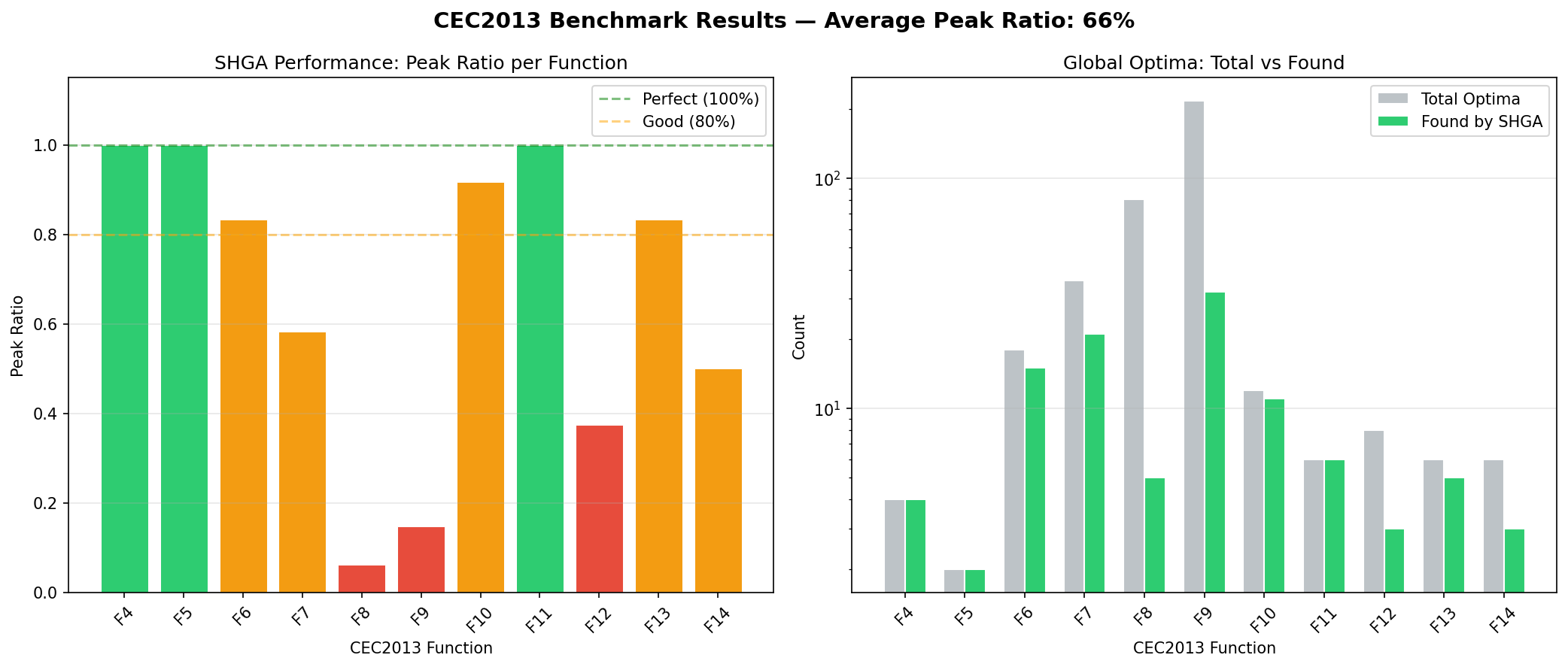
SHGA performance across CEC2013 functions F4-F14. Left: Peak Ratio per function (green = perfect, orange = partial, red = poor). Right: found vs total optima count. The algorithm achieves perfect scores on low-dimensional functions and partial coverage on higher-dimensional compositions.

Keypoints

• Peak Ratio (PR) is the primary metric: fraction of optima found

• Compute PR at multiple accuracy levels (1e-1 to 1e-5)

• Visualize 2D solutions with contour plots

• Track convergence over iterations

• PR = 1.0 means all known optima were found