PINN Methodology

Objectives

• Understand the electrochemistry behind PEM voltage prediction

• Learn about the Teacher-Student PINN architecture

• Know why knowledge distillation improves OOD generalization

• Understand the role of each physics parameter

• Know why baseline comparisons matter for validating the physics approach

Why This Matters

The Scenario: A control systems engineer is designing a model predictive controller (MPC) for a PEM electrolyzer stack. She needs a voltage model that runs in under 5 ms per prediction, respects known electrochemistry (Nernst, Butler-Volmer, Ohmic losses), and doesn’t produce nonsense at high pressures the stack hasn’t been tested at yet. A pure neural network is fast but unreliable outside training data; a full CFD simulation is accurate but takes hours.

The Research Question: Does embedding electrochemical equations directly into the model architecture — rather than hoping a neural network learns the physics from data alone — produce measurably better out-of-distribution generalization? And how much of a large teacher model’s knowledge can be compressed into just 12 physics parameters?

What This Episode Gives You: The electrochemistry behind every term in the voltage equation, the teacher-student architecture, and why each training choice (SGD vs Adam, different schedulers) was made.

Voltage Decomposition

The total cell voltage is the sum of multiple components:

V_cell = V_rev + V_act + V_ohm + V_conc + V_corr

Where:

• V_rev: Reversible (Nernst) voltage - thermodynamic minimum

• V_act: Activation overpotential - kinetic losses (anode + cathode)

• V_ohm: Ohmic overpotential - resistance losses

• V_conc: Concentration overpotential - mass transport losses

• V_corr: Hybrid correction - small logistic correction (clamped to +/-100 mV)

1. Nernst Equation (Reversible Voltage)

V_rev = 1.229 - 0.9x10^-3(T - 298.15) + (RT/nF) x ln(P_H2 x sqrt(P_O2) / P_H2O)

2. Butler-Volmer (Activation Overpotential)

eta_act = (RT / alphanF) x arcsinh(i / 2*i0)

Separate anode and cathode contributions with individual transfer coefficients (alpha_a, alpha_c) and exchange current densities (i0_a, i0_c). Exchange currents use Arrhenius temperature scaling.

3. Ohmic Loss

V_ohm = i x R_ohm

Temperature-dependent resistance with Arrhenius scaling: R_ohm = R_ohm_ref x exp(-E_R/R x (1/T - 1/T_ref)).

4. Concentration Overpotential

eta_conc = -(RT/nF) x ln(1 - i/i_lim)

Where i_lim depends on pressure via Fick’s law and temperature via diffusion scaling.

5. Hybrid Correction

delta_corr = clamp( (a x sigmoid(b x (i - c)) + d) x (1 + p x dP/P_ref + t x dT/T_ref), +/-0.1V )

A small logistic correction with pressure and temperature modulation, accounting for effects not captured by the first four terms.

6-Model Comparison Framework

The notebook trains 6 models to answer the key question: does embedding physics help generalization, or can a large enough neural network learn the physics from data alone?

Pure ML Baselines (No Physics)

Model	Architecture	Parameters
PureMLP	[4 -> 128 -> 64 -> 1]	~2,000
BigMLP	[4 -> 256 -> 128 -> 64 -> 1]	~50,000
Transformer	Self-attention + MLP	~50,000

All baselines use SGD + CosineAnnealingLR + early stopping for a fair comparison.

Physics-Informed Models

Model	Architecture	Parameters	Training
Teacher	Physics equations + MLP residual	~9,000	SGD on labels
Pure Physics	Physics equations + logistic correction	12	Adam on labels only (alpha=1.0)
Distilled Student	Physics equations + logistic correction	12	Adam on 10% labels + 90% teacher

Teacher Model: HybridPhysicsMLP

The teacher combines physics equations with an MLP residual:

• 8 learnable physics parameters: exchange currents, resistance, transfer coefficients, corrections

• MLP residual: [4 -> 128 -> 64 -> 1] with LayerNorm, GELU, Dropout

• Total: ~9,354 parameters

• Training: SGD optimizer (NOT Adam!) + CosineAnnealingLR

The MLP correction is clamped to +/-100 mV to prevent overfitting.

Why SGD Over Adam?

Adam adapts learning rates per-parameter, which can overfit to IID validation data. SGD with momentum provides smoother optimization landscapes and better OOD generalization. This is demonstrated empirically in the ablation study (notebook Part 9).

Student Model: PhysicsHybrid12Param

The student is a pure physics model with hybrid corrections:

• 6 learnable physics parameters: i_lim_ref, i0_a_ref, i0_c_ref, R_ohm_ref, alpha_a, alpha_c

• 6 fixed physics constants (registered as non-learnable buffers):

Constant	Symbol	Value	Source
Anode activation energy	E_a,a	50 kJ/mol	Literature (Ir catalysts)
Cathode activation energy	E_a,c	60 kJ/mol	Literature (Pt catalysts)
Ohmic activation energy	E_R	15 kJ/mol	Literature (Nafion membrane)
Temperature exponent	gamma	0.2	Empirical
Pressure exponent (Fick’s law)	beta	0.7	Fick’s law scaling
Reference temperature	T_ref	353.15 K (80°C)	Experimental design

• 6 learnable hybrid corrections: logistic function with pressure/temperature modulation

• Total: 12 learnable parameters

Parameter Constraints

Physics parameters use constrained representations to guarantee physically valid values:

• Positive quantities (exchange currents, resistance, limiting current): stored in log-space, exponentiated at runtime

• Transfer coefficients: stored as raw values, mapped through sigmoid to [0.3, 1.0]

Knowledge Distillation

The student is trained with a combined loss:

Loss = alpha x MSE(student, labels) + (1-alpha) x MSE(student, teacher)

With alpha = 0.1 (10% labels, 90% teacher), the student learns the teacher’s implicit physics understanding, resulting in better OOD generalization with far fewer parameters.

Pure Physics vs Distilled Student

Both have the same 12-parameter architecture. The only difference is training:

• Pure Physics (alpha=1.0): learns from labels only, no teacher signal

• Distilled Student (alpha=0.1): learns 90% from teacher, which acts as a regularizer

The distillation benefit is typically 5-10 mV improvement in OOD performance.

Training Configuration

The teacher and student use deliberately different training configurations. These choices are empirically validated in the ablation study (notebook Part 9).

Teacher Training

Setting	Value	Rationale
Optimizer	SGD(lr=0.01, momentum=0.9, weight_decay=1e-4)	Smoother optimization prevents MLP overfitting
Scheduler	CosineAnnealingLR(T_max=epochs, eta_min=0.0001)	Gradual decay to fine learning rate
Loss	MSE (mean squared error, in Volts)	Standard regression loss
Epochs	100	Sufficient for convergence with early stopping
Early stopping	patience=30	Stops 30 epochs after last improvement
Gradient clipping	max_norm=1.0	Prevents exploding gradients from physics terms
Validation metric	MAE in millivolts	More interpretable than MSE for comparison

The teacher typically converges early (best epoch ~17-30) and early stopping terminates training well before 100 epochs.

Student Training

Setting	Value	Rationale
Optimizer	Adam(lr=0.001, weight_decay=1e-5)	Adaptive rates help sparse 12-param model converge
Scheduler	ReduceLROnPlateau(factor=0.5, patience=10)	Halves LR when validation stalls for 10 epochs
Loss	alpha x MSE(student, labels) + (1-alpha) x MSE(student, teacher)	Combined distillation loss
Epochs	200	More epochs needed for plateau-based scheduling
Early stopping	patience=40	Longer patience since ReduceLROnPlateau needs time
Gradient clipping	max_norm=1.0	Same as teacher
Validation metric	MAE in millivolts	Same as teacher

Why Different Optimizers?

The teacher has ~9,000 parameters including an MLP with weight matrices. SGD with momentum prevents the MLP from overfitting to training-specific patterns, which is critical for OOD generalization. This is the single most impactful training choice, as shown in the ablation study.

The student has only 12 constrained physics parameters (stored in log-space or sigmoid-bounded). Adam’s per-parameter adaptive learning rates help these sparse, heterogeneous parameters converge efficiently. Since the student has no MLP, the overfitting risk that SGD addresses does not apply.

Baseline Training

All pure-ML baselines (PureMLP, BigMLP, Transformer) use the same configuration as the teacher for fair comparison:

• SGD(lr=0.01, momentum=0.9, weight_decay=1e-4) + CosineAnnealingLR

• 100 epochs, patience=30, gradient clipping max_norm=1.0

This ensures differences in OOD performance are due to architecture (physics vs no physics), not training choices.

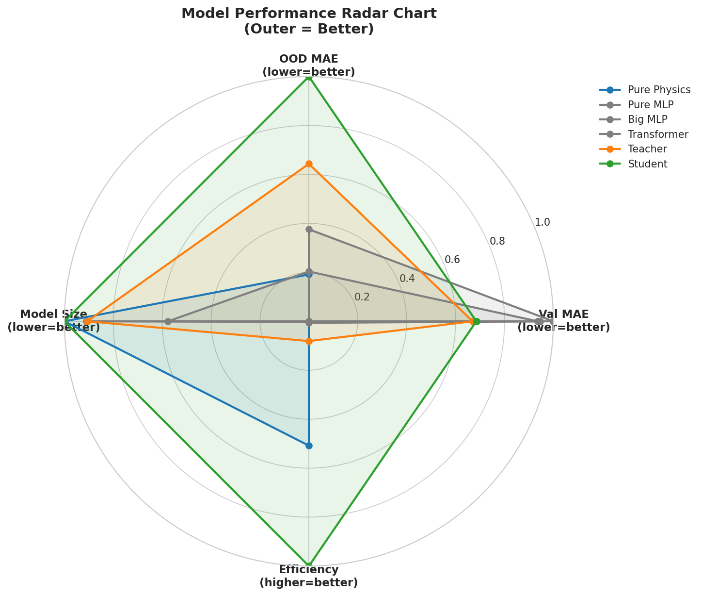
Multi-dimensional radar comparison of all 6 models. The student (green) achieves the best overall balance across accuracy, OOD generalization, and model simplicity.

The 12-Number Equation

After training, the distilled student reduces to a closed-form equation:

V_cell = E_nernst(T, P_H2, P_O2) + eta_act_a(i, T) + eta_act_c(i, T)
       + eta_ohm(i, T) + eta_conc(i, T, P) + delta_corr(i, T, P)

Each term is an explicit function of operating conditions and the 12 learned constants. The notebook (Part 11) implements this as a standalone NumPy function and verifies it matches the PyTorch model to micro-volt precision. This means:

• No neural network at deployment

• Reproducible in any programming language or spreadsheet

• Every parameter has direct physical interpretation

• The model can be published as a table of 12 numbers

Keypoints

• Cell voltage = V_rev + V_act + V_ohm + V_conc + V_corr (5 physical components)

• 6 models compared: 3 pure-ML baselines + teacher + pure physics + distilled student

• Teacher: SGD + CosineAnnealingLR, 100 epochs, patience=30

• Student: Adam + ReduceLROnPlateau, 200 epochs, patience=40

• Different optimizers for different architectures: SGD prevents MLP overfitting, Adam helps sparse physics params

• All baselines use SGD for fair comparison

• Gradient clipping (max_norm=1.0) stabilizes physics-constrained training

• MSE for training loss, MAE in mV for evaluation

• Knowledge distillation with alpha=0.1 transfers physics understanding

• The trained student IS a deterministic equation, reproducible from 12 numbers

• Keep-out validation ensures the model generalizes to unseen conditions