Running Experiments

Objectives

• Run the training pipeline from the command line

• Understand the different execution modes

• Use tmux and tee for long-running experiments with logging

• Interpret training output: tqdm progress bars, dual losses, early stopping

• Understand the two ablation studies (CLI architecture comparison vs notebook hyperparameter sweep)

• Navigate the 11-part interactive notebook

Why This Matters

The Scenario: An ML engineer has trained a voltage prediction model that scores 5 mV error on validation data — impressive on paper. But when the hydrogen plant starts operating at 40 bar (a pressure never seen in training), predictions are off by 50 mV. The model memorized the training distribution instead of learning the underlying physics. She needs a training pipeline that proves the model generalizes before deployment.

The Research Question: How do you train and validate 6 different model architectures on the same data with a fair comparison, and how do you use keep-out conditions to measure real generalization rather than just in-distribution accuracy?

What This Episode Gives You: The complete training pipeline — CLI commands, notebook walkthrough, ablation studies, and how to interpret the OOD metrics that actually matter.

Usage

1. Activate the Environment

cd ~/wp7-UC2-pem-electrolyzer-digital-twin
source venv/bin/activate

2. Run the Main Training Script

python scripts/pem_electrolyzer/main.py \
    --mode full \
    --device cuda \
    --epochs 100

3. Interactive Exploration with Jupyter

jupyter lab --no-browser --ip=127.0.0.1 --port=8888
# Open demonstrator-v1.orchestrator.ipynb

Command Line Options

Option	Default	Description
--mode	full	Execution mode: full, quick-test, teacher-only, ablation
--data-dir	dataset/	Path to dataset directory
--output-dir	results/	Path to output directory
--epochs	100	Training epochs
--seed	42	Random seed
--alpha	0.1	Distillation alpha (0.1 = 90% teacher, 10% data)
--batch-size	4096	Batch size
--lr	0.01	Learning rate
--device	auto	Device: cuda, cpu, or auto

Example Experiments

Quick Test (Recommended First)

Run 5 epochs to verify everything works:

python scripts/pem_electrolyzer/main.py --mode quick-test

Full Training Pipeline

Train teacher, distill student, train baselines, and run all evaluations:

python scripts/pem_electrolyzer/main.py --mode full --device cuda --epochs 100

Teacher Only

Train just the physics-hybrid teacher model:

python scripts/pem_electrolyzer/main.py --mode teacher-only --epochs 50 --seed 42

Ablation Study

Run all 7 ablation experiments across 3 seeds (21 total runs):

python scripts/pem_electrolyzer/main.py --mode ablation --device cuda

Custom Learning Rate and Batch Size

python scripts/pem_electrolyzer/main.py --mode full --lr 0.001 --batch-size 2048 --epochs 200

CPU-Only Training

python scripts/pem_electrolyzer/main.py --mode full --device cpu --epochs 50

Reproducibility with Fixed Seed

python scripts/pem_electrolyzer/main.py --mode full --seed 123 --epochs 100

Background Training (Long Runs)

For long-running experiments, use tmux with tee for simultaneous terminal output and logging:

# Start background training with logging
tmux new -s training 'python scripts/pem_electrolyzer/main.py \
    --mode full --device cuda --epochs 100 2>&1 | tee training.log'

# Monitor progress from another terminal
tail -f training.log

# Attach to the tmux session
tmux attach -t training

# Detach from session: Ctrl+B, then D

The 2>&1 | tee training.log construct captures both stdout and stderr to the log file while still displaying output in the terminal. This is useful for:

• Reviewing training progress after disconnection

• Debugging errors that occurred during training

• Sharing training logs with collaborators

Expected Training Output

Training uses tqdm progress bars for clean output. When running --mode full, you should see:

=== PEM Electrolyzer PINN Training ===
Device: cuda (NVIDIA A100)

============================================================
Loading Test4 Training Data (STRICT + KEEP-OUT split)
============================================================
Raw samples: 193,248
After strict filtering: 15,234 (7.9%)
KEEP-OUT validation split (76-80C):
  Training: 11,534 samples (75.7%)
  Validation: 3,700 samples (24.3%)

--- Training Teacher (HybridPhysicsMLP) ---
Teacher: |████████████████████| 100/100 [01:02<00:00] loss=0.00032 val=13.9mV best=13.9mV lr=0.00010 *

--- Training Baselines ---
Training pure_mlp (2,049 params)...
Training big_mlp (43,393 params)...
Training transformer (529,793 params)...

--- Distilling Student (PhysicsHybrid12Param) ---
Student: |███████████████     | 152/200 [01:18<00:24] Early stop @ 152 | best=13.8mV

--- OOD Evaluation (All 6 Models) ---
FULL MODEL COMPARISON (All 6 Models)
==========================================================================
Model                Params   Val (mV)  Test2 (mV)  Test3 (mV)  OOD Avg (mV)
--------------------------------------------------------------------------
Distilled Student        12     13.8        14.7        15.9          15.3
Teacher               9354     13.9        42.5        13.8          28.2
Pure Physics             12     25.1        18.3        22.7          20.5
PureMLP               2049     12.5        45.2        38.1          41.7
BigMLP               43393     11.8        52.3        41.5          46.9
Transformer         529793     10.2        68.4        55.2          61.8

Results saved to results/results.json

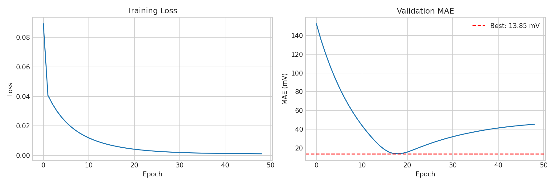
Real training curves from the teacher model: (Left) MSE loss decreasing smoothly over epochs. (Right) Validation MAE converging to 13.85 mV best, with the dashed red line marking the best checkpoint.

Key observations from the output:

• Teacher converges early (typically best at epoch ~17) with early stopping patience of 30

• Student training shows label loss (L) and distillation loss (D) separately

• Progress bars use tqdm with real-time postfix: loss, validation MAE, best MAE, learning rate

• A * after the postfix indicates a new best epoch was found

• The 6-model comparison table shows all models sorted by OOD Average MAE

• The distilled student (12 params) typically beats all larger models on OOD

If you see CUDA not available, falling back to CPU, GPU drivers may not be installed correctly. See Episode 03 for troubleshooting.

Training Deep Dive

What Happens During --mode full

The full pipeline executes these steps in order:

1. Load and filter data: Load Test4 CSV, apply strict filtering (removes out-of-range samples), split into train/validation using 76-80C keep-out

2. Train teacher (HybridPhysicsMLP): SGD optimizer, CosineAnnealingLR, 100 epochs with early stopping (patience=30)

3. Train baselines: PureMLP, BigMLP, Transformer — each with the same SGD config for fair comparison

4. Distill student (PhysicsHybrid12Param): Adam optimizer, ReduceLROnPlateau, 200 epochs (patience=40), alpha=0.1

5. Train pure physics: Same student architecture but alpha=1.0 (no teacher signal)

6. OOD evaluation: Evaluate all 6 models on Test2 and Test3 datasets

Reading the Progress Bar

The tqdm progress bar shows real-time training metrics:

Teacher: |████████████████████| 100/100 [01:02<00:00] loss=0.00032 val=13.9mV best=13.9mV lr=0.00010 *

Field	Meaning
loss=0.00032	Training MSE loss (in Volts squared). Lower is better.
val=13.9mV	Current epoch’s validation MAE (in millivolts)
best=13.9mV	Best validation MAE seen so far across all epochs
lr=0.00010	Current learning rate (decreases via scheduler)
*	This epoch achieved a new best validation MAE

For the student, the progress bar also shows dual losses:

Student: |███████████████     | 152/200 [01:18<00:24] L=0.00045 D=0.00032 val=13.8mV best=13.8mV

Field	Meaning
L=0.00045	Label loss: MSE(student predictions, true labels)
D=0.00032	Distillation loss: MSE(student predictions, teacher predictions)

With alpha=0.1, the total loss is 0.1 x L + 0.9 x D. The distillation loss (D) typically dominates.

Early Stopping Behavior

Training does not always run for the full epoch count:

• Teacher: Typically converges at epoch ~17-30 (patience=30 means it runs 30 more epochs after the best, then stops)

• Student: May early-stop around epoch 100-160 (patience=40)

• Baselines: Variable — simpler models converge faster, Transformer may use more epochs

When early stopping triggers, the progress bar shows: Early stop @ 152 | best=13.8mV

The best model checkpoint is saved at the epoch with the lowest validation MAE, not the final epoch.

Learning Rate Schedules

Two different schedules are used:

CosineAnnealingLR (teacher and baselines): Smoothly decreases the learning rate from 0.01 to 0.0001 following a cosine curve over the full epoch count. This provides gradual refinement.

ReduceLROnPlateau (student): Starts at 0.001 and halves the learning rate whenever validation MAE does not improve for 10 consecutive epochs. This adapts to the student’s convergence speed.

Ablation Studies

There are two distinct ablation studies — one for the CLI and one for the notebook. They test different hypotheses.

CLI Ablation (--mode ablation)

Compares model architectures to prove physics-informed models generalize better than pure ML:

python scripts/pem_electrolyzer/main.py --mode ablation --device cuda

#	Experiment	What It Tests
1	pure_mlp	Small MLP baseline (~2K params, no physics)
2	big_mlp	Large MLP baseline (~43K params, no physics)
3	transformer	Attention-based baseline (~530K params, no physics)
4	teacher	Physics-hybrid teacher (~9K params)
5	pure_physics	Student with alpha=1.0 (12 params, no teacher signal)
6	student_keepout	Student with alpha=0.1, keep-out validation
7	student_random	Student with alpha=0.1, random validation

Each experiment runs across 3 seeds [42, 91, 142] = 21 total runs. Results are saved to results/ablation/ with per-experiment JSON files.

Key question answered: Does physics help, or can a large enough network learn it from data?

Notebook Ablation (Part 9)

Compares hyperparameter choices to show which training decisions matter most:

#	Experiment	What It Tests
1	baseline	Default config: SGD + keep-out + lr=0.01
2	no_keepout	Temperature keep-out disabled
3	random_val	80/20 random validation split
4	adam	Adam optimizer instead of SGD
5	low_lr	Learning rate 0.001 (10x lower)
6	high_lr	Learning rate 0.05 (5x higher)
7	no_wd	No weight decay (weight_decay=0)

Each experiment runs across 3 seeds [42, 123, 456] = 21 total runs. Disabled by default — set RUN_ABLATION = True in the notebook to run.

Key question answered: Which training choices matter most for OOD generalization?

Expected Ablation Insights

The paper quantifies three complementary mechanisms that contribute to the student’s OOD performance:

Mechanism	Improvement	Comparison
Physics constraints	56%	Pure MLP (35.1 mV) → Student (15.3 mV)
Knowledge distillation	50%	Pure Physics (30.6 mV) → Student (15.3 mV)
Keep-out validation	29%	Random val (22.3 mV) → Keep-out (15.9 mV)

Additional insights:

• SGD beats Adam for the teacher by ~10-15 mV on OOD

• Weight decay has a modest effect (~2-3 mV)

• Learning rate sensitivity is moderate — 0.01 is near-optimal; 0.05 can diverge, 0.001 converges slowly

• Architecture matters most: the 12-param student beats ~530K-param baselines regardless of hyperparameters

Reproducibility Across Seeds

Results are stable across random seeds [42, 91, 142]:

Model	OOD Avg (mean ± std)
Distilled Student	15.9 ± 1.0 mV
Teacher	28.2 ± 1.5 mV
Pure MLP	35.1 ± 2.3 mV
Transformer	39.0 ± 3.1 mV

The worst Student seed (17.1 mV) still beats the best Transformer seed (37.2 mV), confirming that the physics-informed approach is robust to initialization.

Notebook Walkthrough (11 Parts)

The interactive notebook (demonstrator-v1.orchestrator.ipynb) covers the full pipeline in 11 parts:

Part	What Happens	Key Output
1	Environment setup	GPU check, imports
2	Data exploration	Distribution plots, filtering statistics
3	PINN methodology	Voltage decomposition stacked area chart
4	Teacher training	tqdm progress bar, training curves, best epoch
5	Baseline comparison	Train PureMLP, BigMLP, Transformer, Pure Physics; 5-model bar chart
6	Knowledge distillation	Student training with label/distillation loss breakdown
7	6-model comparison	Full comparison table + bar chart + residual distribution
8	Interactive widgets	Configure and launch experiments with dropdown controls
9	Ablation study	Systematic parameter sweeps (optional, set RUN_ABLATION=True)
10	Summary	Model ranking, next steps
11	12-number equation	Extract 12 params, NumPy implementation, verification, polarization curves

Part 11: The Biggest Takeaway

Part 11 is the culmination of the entire notebook. It demonstrates that:

1. The trained student is defined by exactly 12 scalar constants

2. A standalone NumPy function reproduces the model with zero PyTorch dependencies

3. The NumPy function matches PyTorch model.forward() to micro-volt precision

4. Full voltage decomposition is computed step-by-step for sample operating conditions

5. Polarization curves are generated showing temperature and pressure effects

6. A reproducibility card lists all constants ready to copy-paste

Result File Format

Results are saved to results/results.json with this structure:

Field	Type	Description
timestamp	string	Training timestamp
config	object	Training configuration (seed, epochs, lr, alpha, device)
teacher	object	Teacher metrics (val_mae_mV, test2_mae_mV, test3_mae_mV, ood_avg_mV)
student	object	Student metrics + learned physics and hybrid parameters

The student section includes the 12 learned parameters:

{
  "student": {
    "val_mae_mV": 13.81,
    "test2_mae_mV": 14.67,
    "test3_mae_mV": 15.91,
    "ood_avg_mV": 15.29,
    "physics_params": {
      "i_lim_ref": 1.293,
      "i0_a_ref": 8.075e-05,
      "i0_c_ref": 0.003470,
      "R_ohm_ref": 0.9947,
      "alpha_a": 0.6375,
      "alpha_c": 0.6710
    },
    "hybrid_params": {
      "corr_a": 0.03471,
      "corr_b": 0.6046,
      "corr_c": 0.6341,
      "corr_d": 0.02045,
      "corr_p": 1.8518,
      "corr_t": 0.3209
    }
  }
}

These 12 numbers are all that is needed to reproduce the model’s predictions without retraining. See Episode 07 for how to use them.

Keypoints

• Always run --mode quick-test first to verify setup

• Use --device cuda for GPU training (much faster)

• Use tmux with tee for long-running experiments with logging

• Training uses tqdm progress bars: watch for loss, val, best, lr, and * (new best)

• Student shows dual losses: L (label) and D (distillation), weighted by alpha

• Early stopping saves the best checkpoint, not the final epoch

• Two ablation studies: CLI compares architectures (7 experiments x 3 seeds), notebook compares hyperparameters (7 x 3)

• Keep-out validation is the single most important training choice for OOD

• The notebook has 11 parts: Parts 5 and 7 compare all 6 models, Part 9 is ablation, Part 11 is the 12-number equation

• Results include 12 learned parameters in results.json for full reproducibility