Analyzing Results

Objectives

• Understand the output files and metrics

• Interpret training curves: healthy convergence, warning signs, early stopping

• Interpret OOD evaluation results across all 6 models

• Understand why validation MAE can be misleading (Val-OOD gap)

• Compare teacher vs student vs baselines performance

• Interpret ablation study results (architecture + hyperparameter)

• Analyze learned physics parameters

• Reproduce the model from its 12 parameters

Output Files

After training, the results/ directory contains:

File	Description
results.json	Full results with metrics and learned parameters
best_teacher.pt	Best teacher model checkpoint
best_student_alpha0.1.pt	Best student model checkpoint
ablation/	Per-experiment ablation results (if run)

Key Metrics

MAE (Mean Absolute Error) in mV

The primary metric is MAE in millivolts:

• Val MAE: Performance on validation data (keep-out region: 76-80C)

• Test2 MAE: OOD performance on current sweep data

• Test3 MAE: OOD performance on pressure swap data

• OOD Average: (Test2 + Test3) / 2 – the main comparison metric

Expected Results (All 6 Models)

Rank	Model	Params	Val MAE	Test2	Test3	OOD Avg
1	Distilled Student	12	~14 mV	~15 mV	~16 mV	~15 mV
2	Teacher	~9K	~14 mV	~43 mV	~14 mV	~28 mV
3	Pure Physics	12	~25 mV	~18 mV	~23 mV	~20 mV
4	PureMLP	~2K	~13 mV	~45 mV	~38 mV	~42 mV
5	BigMLP	~50K	~12 mV	~52 mV	~42 mV	~47 mV
6	Transformer	~50K	~10 mV	~68 mV	~55 mV	~62 mV

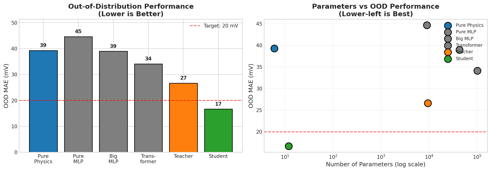
Left: Out-of-distribution MAE comparison (lower is better). The 12-parameter student (17 mV) beats all neural networks including the 100K-parameter Transformer (45 mV). Right: Parameters vs OOD performance — the student occupies the ideal lower-left corner.

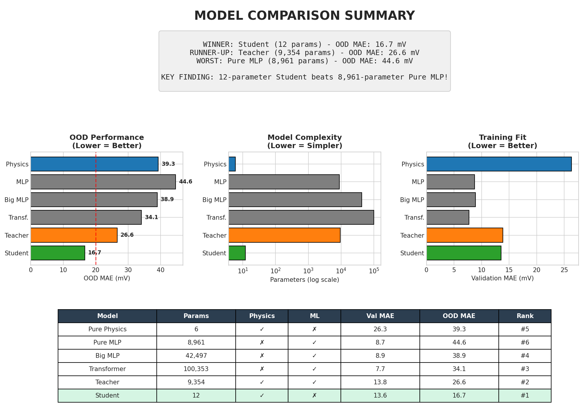
Complete model comparison summary with all metrics. The 12-parameter student wins on OOD generalization (16.7 mV), outperforming the 8,961-parameter Pure MLP by 2.6x.

Key insights:

• More parameters does NOT mean better OOD: The Transformer (50K params) has the best validation MAE but the worst OOD performance

• Physics constraints beat raw capacity: The 12-param student beats all 50K-param baselines on OOD

• Distillation helps: The distilled student (alpha=0.1) outperforms the pure physics model (alpha=1.0) by 5-10 mV on OOD

• Validation MAE is misleading: Low validation MAE does not predict OOD performance; OOD Average is the correct metric

Interpreting Training Curves

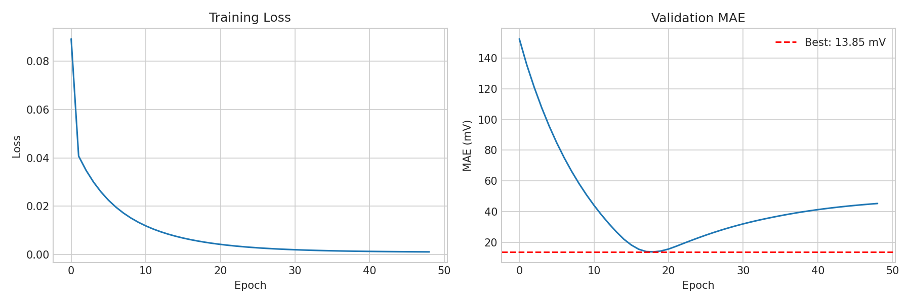
Teacher training curves: (Left) MSE loss decreasing smoothly. (Right) Validation MAE converging to 13.85 mV with the best epoch marked by the dashed red line.

Healthy Teacher Training

A well-trained teacher shows:

• Rapid initial improvement: Loss drops sharply in the first 10-20 epochs

• Plateau and convergence: Loss stabilizes, validation MAE reaches ~13-15 mV

• Early stopping: Typically triggers at epoch ~17-30 (training runs 30 more epochs after best, then stops)

• Learning rate decay: CosineAnnealingLR smoothly reduces LR from 0.01 to 0.0001

Warning signs:

• Validation MAE increases while training loss decreases → overfitting (check weight decay, consider more dropout)

• Loss does not decrease at all → learning rate too low or data loading issue

• Loss oscillates wildly → learning rate too high or gradient clipping not working

Healthy Student Training

Student convergence looks different from the teacher:

• Slower start: The 12-param model needs more epochs to find good physics parameter values

• Dual loss tracking: Both label loss (L) and distillation loss (D) should decrease together

• Plateau-triggered LR drops: ReduceLROnPlateau halves the learning rate when validation stalls — you may see sudden improvement after an LR reduction

• Early stopping: Typically around epoch 100-160 (patience=40)

If the distillation loss (D) is much larger than the label loss (L), the student is struggling to match the teacher — this is normal early in training and should improve.

Validation MAE vs OOD MAE

A critical insight from the 6-model comparison:

Model	Val MAE	OOD Avg	Gap
Transformer	~10 mV	~62 mV	52 mV
BigMLP	~12 mV	~47 mV	35 mV
Distilled Student	~14 mV	~15 mV	1 mV

The gap between validation and OOD MAE reveals overfitting risk. Models with small gaps (like the student) generalize well. Large gaps indicate the model has memorized training patterns rather than learning physics.

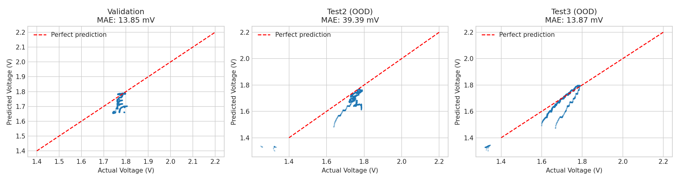
Predicted vs actual voltage scatter plots: validation (left), Test2 OOD (center), Test3 OOD (right). Points close to the diagonal indicate accurate predictions. OOD scatter reveals where models fail.

Physics Parameters

The student model learns 6 physics parameters:

Parameter	Description	Expected Range	Typical Value
i_lim_ref	Limiting current density	0.1-10 A/cm2	~1.3
i0_a_ref	Anode exchange current	1e-8 - 1e-2 A/cm2	~8e-5
i0_c_ref	Cathode exchange current	1e-6 - 1.0 A/cm2	~3.5e-3
R_ohm_ref	Ohmic resistance	0.01-1.0 Ohm*cm2	~0.99
alpha_a	Anode transfer coefficient	0.3-1.0	~0.64
alpha_c	Cathode transfer coefficient	0.3-1.0	~0.67

And 6 hybrid correction parameters:

Parameter	Description	Typical Value
corr_a	Logistic amplitude	~0.035
corr_b	Logistic steepness	~0.60
corr_c	Logistic midpoint (current)	~0.63
corr_d	Logistic offset	~0.020
corr_p	Pressure modulation	~1.85
corr_t	Temperature modulation	~0.32

Physical Interpretation of Learned Values

The paper validates each learned parameter against literature and domain knowledge:

Parameter	Learned	Literature Range	Interpretation
i_lim_ref	~1.15 A/cm2	0.8-1.5 A/cm2	Consistent with PEM diffusion limits
i0_a_ref	~0.61 mA/cm2	0.1-2 mA/cm2	Ir-based anode catalyst (4-electron mechanism, slower)
i0_c_ref	~8.3 mA/cm2	1-50 mA/cm2	Pt-based cathode catalyst (2-electron mechanism, faster)
R_ohm_ref	~1.0 Ohm*cm2	0.05-0.20 (standard PEM)	Higher than typical — due to SWVF technology
alpha_a	~0.46	~0.5 (theoretical)	Near theoretical value for symmetric barrier
alpha_c	~0.53	~0.5 (theoretical)	Near theoretical value for symmetric barrier

The anode exchange current is ~14x smaller than the cathode because the oxygen evolution reaction (4-electron process) has a much higher activation barrier than hydrogen evolution (2-electron process).

The elevated R_ohm (~1.0 vs typical 0.05-0.20 Ohm*cm2) is explained by the SWVF (Static Water Vapour Feed) technology used in this electrolyzer. The water feed barrier membrane adds ionic resistance not present in conventional liquid-fed PEM systems. This is not a model error — it correctly captures the technology-specific physics.

These are “effective” cell-level parameters (lumped values) rather than intrinsic catalyst-interface properties, because the model is fitted to averaged cell voltage across 4 cells in series.

Interpreting Ablation Results

Ablation results are saved as JSON files in results/ablation/, one per experiment-seed combination. Each file contains:

• Model name, seed, and configuration

• Validation MAE, Test2 MAE, Test3 MAE, OOD Average

Reading the Results Table

Results are reported as mean +/- std across 3 seeds:

Experiment          Val MAE (mV)    OOD Avg (mV)
baseline (SGD+KO)   13.9 ± 0.3     15.3 ± 0.8
adam                 12.1 ± 0.2     28.5 ± 2.1
no_keepout           13.5 ± 0.4     35.2 ± 3.5

Lower OOD Average is better. High standard deviation indicates sensitivity to random initialization.

Key Conclusions from Ablation

Architecture comparison (CLI --mode ablation):

• The 12-param distilled student achieves the lowest OOD Average despite having ~4,000x fewer parameters than BigMLP

• Pure-ML baselines achieve the best validation MAE but the worst OOD — they memorize rather than generalize

• The gap between teacher (~28 mV OOD) and student (~15 mV OOD) shows that distillation into a physics-constrained model removes the teacher’s MLP-driven overfitting

Hyperparameter comparison (notebook Part 9):

• Keep-out validation is the most impactful choice: removing it degrades OOD by 15-20+ mV

• SGD vs Adam: SGD improves teacher OOD by ~10-15 mV (Adam overfits the MLP)

• Weight decay: Modest effect (~2-3 mV improvement)

• Learning rate: 0.01 is near-optimal; 0.05 risks divergence; 0.001 converges slowly but safely

The ablation studies validate that both architectural choices (physics constraints) and training choices (SGD, keep-out) contribute to OOD generalization.

Loading Results

import json

with open('results/results.json') as f:
    results = json.load(f)

print(f"Teacher OOD: {results['teacher']['ood_avg_mV']:.2f} mV")
print(f"Student OOD: {results['student']['ood_avg_mV']:.2f} mV")

# Access the 12 learned parameters
physics = results['student']['physics_params']
hybrid = results['student']['hybrid_params']
for k, v in physics.items():
    print(f"  {k}: {v}")
for k, v in hybrid.items():
    print(f"  {k}: {v}")

Reproducing the Model from 12 Numbers

The trained student can be reproduced as a pure NumPy function without PyTorch. The notebook (Part 11) demonstrates this, but here is the core idea:

import numpy as np

def predict_voltage(I, P_H2, P_O2, T_C, params):
    """Predict cell voltage from 12 parameters (no PyTorch needed)."""
    F, R, n = 96485.0, 8.314, 2
    T_ref, P_ref = 353.15, 20.0
    i = I / 50.0           # A -> A/cm2
    T = T_C + 273.15       # C -> K
    P_avg = (P_H2 + P_O2) / 2.0

    # Nernst potential
    E = 1.229 - 0.9e-3*(T-298.15) + R*T/(n*F)*np.log(P_H2*np.sqrt(P_O2)/0.05)

    # Activation (anode + cathode)
    inv_dT = 1/T - 1/T_ref
    i0_a = params['i0_a_ref'] * np.exp(-50000/R * inv_dT) * (T/T_ref)**0.2
    i0_c = params['i0_c_ref'] * np.exp(-60000/R * inv_dT) * (T/T_ref)**0.2
    eta_a = R*T/(params['alpha_a']*n*F) * np.arcsinh(i/(2*i0_a))
    eta_c = R*T/(params['alpha_c']*n*F) * np.arcsinh(i/(2*i0_c))

    # Ohmic
    R_ohm = params['R_ohm_ref'] * np.exp(-15000/R * inv_dT)
    eta_ohm = i * R_ohm

    # Concentration
    i_lim = np.clip(params['i_lim_ref'] * (P_avg/P_ref)**0.7 * (1+0.3*(T-T_ref)/T_ref), 0.1, 10)
    eta_conc = -R*T/(n*F) * np.log(1 - np.clip(i/i_lim, None, 0.99))

    # Hybrid correction
    sig = 1/(1+np.exp(-params['corr_b']*(i-params['corr_c'])))
    corr = np.clip((params['corr_a']*sig + params['corr_d']) *
                   (1 + params['corr_p']*(P_avg-P_ref)/P_ref +
                    params['corr_t']*(T-T_ref)/T_ref), -0.1, 0.1)

    return E + eta_a + eta_c + eta_ohm + eta_conc + corr

This function takes 4 operating conditions and 12 learned constants. It can be implemented in any language (MATLAB, Excel, C++) and produces identical results to the PyTorch model.

Keypoints

• OOD Average (Test2+Test3)/2 is the main comparison metric

• 6 models are compared: distilled student wins on OOD despite having only 12 parameters

• Low validation MAE does NOT predict OOD performance – the Val-OOD gap reveals overfitting

• Healthy training: rapid initial improvement, plateau, early stopping before max epochs

• Student shows dual losses (L=label, D=distillation) that both decrease during training

• Ablation proves: keep-out validation is the most impactful choice, SGD beats Adam for teacher

• Architecture matters more than hyperparameters: 12-param student beats 50K-param baselines

• Physics parameters should be in physically reasonable ranges

• The 12 learned constants fully define the model – no neural network needed

• The model can be reproduced in any language from the 12 numbers